Source of the Unknown: Stochastic Engineering and Precision Measurement in the Age of AI Agents

Thesis (one line): In the age of autonomous AI agents, a specification is not a source of truth but a source of a distribution over possible implementations; it becomes an engineering artifact only once its tolerance is measured and written into a precision budget.

Act I: Foreplay (The Sacred Artifact)

For decades, system architects and engineers have built an unshakeable cult around a single concept: the Single Source of Truth. We worshipped it like a sacred artifact. We learned to draw polished, deterministic SysML models, to structure business requirements into beautiful Markdown specifications, and to lock architectural decisions into RFCs.

When such a document sits in the repository, the team feels total control. We believe that because an idea has been recorded in symbols on a screen, we have tamed reality and captured precise engineering intent. This is our comfort zone — a sterile world ruled by the illusion of absolute precision and predictability. We write the text, close the ticket in Jira, and consider the design work done.

Act II: Rising Tension (The Cloud of Intent)

Then comes mid-2026, and the commercialization of autonomous AI agents (think Claude Code or Cursor) pulls a hard about-face. The old deterministic source of truth — with our schemas, compiled code, and rigid boundary lines — quietly collapses into fleeting human “intents” and endless conversational streams in chat windows.

We feed the AI our “perfect” spec, treating it as truth. But a large language model reads text differently than a colleague with ten years of shared context: it doesn’t have our implicit engineering experience, so where a human sees “room for improvisation,” the model sees a hole in the context. And it fills that hole — by sampling from its own probability distribution, delivering the result with a professor’s confidence.

The sacred specification transforms, before our eyes, into a source of the unknown. Here, AI acts as a multiplier of chaos: it takes our hidden disorder and scales it into a spaghetti architecture faster than the team can notice — in tokens, lines of code, and agent iterations that a human operator can no longer comprehend or audit.

An important distinction the industry has lost: the “fog” of a specification is not one disease but at least three distinct failure modes:

Failure mode	What it is	Example
Ambiguity	Several plausible implementations of the same text	“flexibly accept transactions”
Incompleteness	Missing constraints, schemas, acceptance criteria	no `Transaction` schema, no failure modes
Untraceability	A requirement hangs in the air, undecomposed into functions	a slogan with no link to the architecture

Each failure mode is caught by its own metric — more on that in Act V. Without this distinction, “spec precision” remains an abstract incantation.

Act III: Weighing the Options (So What Is Precision, Anyway?)

We find ourselves at a crossroads. The architect faces a fundamental question: if our specifications are fuzzy, what do we even mean by “precision of the source of truth”?

Option A (Old-Believer): Try to write a “perfect” specification in human language. Spend months polishing every comma in Notion or Confluence. Spoiler: it will be stale by evening anyway, and the AI will still find linguistic slack in it to generate architectural debt.
Option B (Prompt Anarchy): Accept the specification as just a bundle of fuzzy wishes. Let the AI vibe freely, play “prompt roulette,” and hope every morning that the latest autonomous refactor didn’t accidentally destroy the system’s logic.
Option C (Escape into Formalism): If natural language is too vague, write the spec in a language whose semantics are unambiguous by construction: first-order logic, TLA+, Alloy, contracts, executable specs. (Romantics will bring up the myth of Sanskrit as “a perfectly unambiguous language for machines” — let’s leave that where it belongs: in nice legends. Living Sanskrit is homonymic and context-dependent, like any natural language.) Formalization genuinely works — but it doesn’t eliminate the unknown, it relocates it: into the choice of abstractions, into model completeness, into the cost of maintaining traceability. And it forces the team to spend years learning notation instead of designing real systems. The slack never disappears — it just moves somewhere harder to see.
Option D (Stochastic / New): Accept the fact that any source of truth has a precision budget — a tolerance the architect sets in advance, the way you set a tolerance on a machined part. Precision will never be binary. A document has its own level of entropy and permissible slack, and our job is not to worship the text as sacred but to set the tolerance explicitly and verify it by measurement. A spec passes the gate not because it “looks fine,” but because its measured slack fits within the declared budget.

Act IV: Climax (The Epiphany of Metrics)

The software industry is stuck in endless arguments about the quality of AI-generated code, while completely ignoring the quality of the knowledge fed into it. We use the word “precision” as an abstract incantation or a humanities-flavored wish.

Without metrics, the term “precision of the source of truth” is completely meaningless.

If you cannot digitize the level of ambiguity in your model or Markdown spec, you are not handing the AI an instruction — you are handing it a lottery ticket. A source of truth without measured precision automatically becomes a source of random results. Precision in AI engineering is not the absence of errors — it is the measured slack of the input document, checked against a budget set in advance.

And every failure mode from Act II gets its own measuring instrument:

Failure mode	Metric	What it catches
Ambiguity	$D_{pair}$, $H_{spec}$ — generation spread	the spread of possible implementations
Incompleteness	$D_{const}$ — constraint density	the lack of machine-readable facts
Untraceability	$K_{drift}$ — relational drift	requirements hanging in mid-air

Act V: Dry Prose (Digitizing the Fog of Specifications)

Architectural case study: how a low-precision Markdown file blows up an AI-agent pipeline

Picture a standard Markdown spec that a business analyst considers a finished requirement:

# User Payment Processing System
1. The system must flexibly accept transactions from various providers.
2. All successful and failed operation results must be logged.

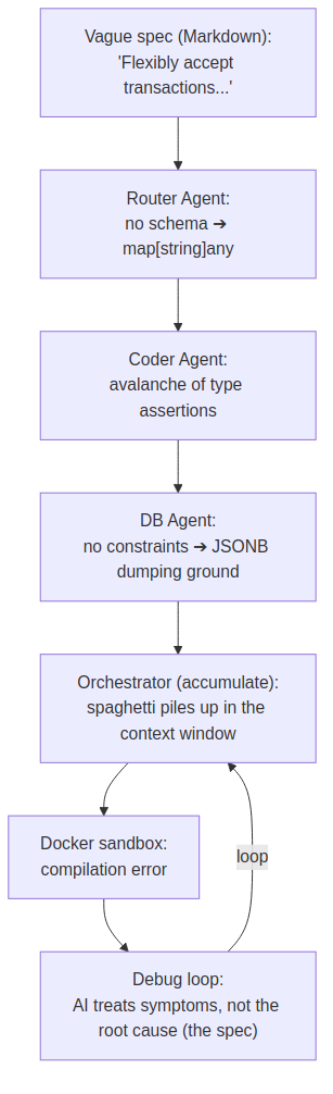
The constraint density of this document is catastrophically low: no schema, no constraint — just adverbs. When we feed this file into an automated orchestration pipeline (say, one built on declarative YAML agent-management topologies), an avalanche of entropy detonates:

Step 1 (Router Agent): Sees the word “flexibly.” Since there are no clear OpenAPI schemas or database constraints in the source, it picks the vaguest possible data structure — map[string]any in Go.
Step 2 (Coder Agent): Receives map[string]any. If the orchestrator’s context mode is set to accumulate (retaining the full history), the model starts generating hundreds of lines of unsafe code full of type assertions, blindly guessing at the transaction’s structure.
Step 3 (Database Agent): Sees the requirement to “log results.” It creates a PostgreSQL table with a JSONB column, into which the AI dumps everything indiscriminately, thoroughly wrecking relational integrity.
Pipeline collapse: By the 4th iteration of the chain, the model’s context window is clogged with generated spaghetti code and lengthy AI apologies. Token consumption grows nonlinearly. When the pipeline tries to assemble this Go code in an isolated Docker sandbox, the compiler throws an interface-mismatch error. The telemetry.jsonl file explodes with recursive errors. The AI falls into an infinite debugging loop, trying to fix code that was built on fog.

Source of the unknown — pipeline collapse from a vague spec

The same case after raising precision

The same business intent, but with explicit constraints:

# User Payment Processing System

@schema Transaction {
  id: UUID,
  amount: Decimal(10,2) @constraint(min: 0.01),
  currency: String(3) @constraint(pattern: "^[A-Z]{3}$"),
  provider: Enum["stripe", "paypal", "adyen"],
  idempotency_key: UUID @constraint(unique)
}

1. [REQ-PAY-01] The system validates the incoming request against the Transaction schema.
   -> [FUN-PAY-01] AcceptTransaction(tx Transaction) (Receipt, error)
2. [REQ-PAY-02] Operation results are recorded in the payment_logs table
   (tx_id UUID FK, status Enum["ok","declined","error"], error_code String?, created_at Timestamp).
   -> [FUN-PAY-02] LogResult(txID, status, errorCode)
3. [REQ-PAY-03] A repeated request with the same idempotency_key returns
   the previous Receipt without charging twice.
   -> [FUN-PAY-03] state machine: received -> authorized -> captured | declined

The difference isn’t in volume — it’s in the number of degrees of freedom we removed from the model’s sampling. The first document permits thousands of incompatible implementations; the second is a narrow corridor. That’s precisely the difference we’re now going to learn to measure.

Engineering metrics for measuring the fog

To keep the orchestrator from releasing AI agents into that death spiral, we’re obligated to first run the source of truth through a system of metrics. Let’s start with the cheapest and most deterministic one.

1. Relational Drift Coefficient ($K_{drift}$) — the deterministic foundation

Measures the number of isolated, “hanging” requirements in the specification’s knowledge graph — ones with no decomposition down to the lower levels of system architecture. The spec is decomposed into a graph following the RFLP paradigm (Requirements, Functional, Logical, Physical), in one of two modes: strict — a deterministic linter over explicit markup ([REQ-*] -> [FUN-*], as in the example above); assisted — a lightweight AI-agent parser with a strict JSON schema on output (Structured Outputs), for when markup doesn’t exist yet. The graph lives in, say, Neo4j.

\[K_{drift} = \frac{\text{Number of Requirements nodes with no outgoing edges to Functional/Logical layers}}{\text{Total number of requirements in the system}}\]

The key property of strict mode: there is no LLM in the measurement loop. It’s a pure graph traversal — deterministic, cheap, reproducible. (In assisted mode, only the traversal itself stays deterministic; the quality of LLM edge extraction is a separate object of validation, and the metric inherits its error.) You can compute it today, without a research lab, and hang it off a git hook. If $K_{drift} > 0.2$ (a threshold — a hypothesis to be calibrated on your own spec corpus), at least a fifth of your “source of truth” consists of abstract slogans that the AI will be forced to implement out of pure invention.

2. Syntactic Constraint Density ($D_{const}$)

Defines the ratio of strictly formalized, machine-readable engineering facts to unbound human prose within the same RFLP graph:

\[D_{const} = \frac{\text{Number of strictly typed relations (must\_satisfy, performs, flows\_to)}}{\text{Total number of unstructured text nodes}}\]

A high $D_{const}$ substantially narrows the space for uncontrolled interpretation: it’s harder for a model to invent nonexistent fields when every entity is pinned down by a schema.

An honest caveat about density: the metric doesn’t penalize prose in general — it penalizes prose not tied to any constraint. A good specification with an elaborated rationale and trade-off analysis will have a lower “raw” density than a bare dump of schemas — and that’s fine. The goal isn’t to maximize $D_{const}$; it’s to remove nodes that yield no typed edge at all. So in CI it’s smarter to normalize density per requirement rather than per whole document.

3. Generation Spread ($D_{pair}$) and Interpretation Entropy ($H_{spec}$)

The most ambitious metric: we measure a document’s ambiguity through the language model’s own reaction to it. The lineage of this trick is honest and well known — it’s self-consistency sampling from the LLM-uncertainty-estimation toolbox, just turned around: aimed not at the model’s answer, but at the input document. But it’s easy to build an instrument that measures its own noise and passes it off as the specification’s signal — hence a strict protocol.

Measurement protocol:

Fix the measurement configuration: model + version, system prompt, temperature, $N$ samples. The metric is only meaningful relative to this configuration — changing the model shifts the entire scale.
Generate $N$ (e.g., 10) variants of the system’s interfaces (Go structs or migration schemas) from the same spec.
Normalize the results to an AST and compute pairwise similarity (in our implementation — a bag of features: types, fields with their types, function signatures → cosine similarity; this is structural similarity of the generated artifacts, not semantic equivalence).
Cluster: results with similarity above a threshold (e.g., 0.95) belong to one equivalence class $x_i$. Then $P(x_i) = x_i / N$.
Compute the interpretation entropy:

\[H_{spec} = - \sum_{i=1}^{n} P(x_i) \log_2 P(x_i)\]

All $N$ variants fall into one cluster ➔ $H_{spec} \to 0$: the interpretation corridor is narrow.
Every generation is its own cluster ➔ $H_{spec} \to \log_2 N$: the document is vague, and releasing it into code generation without further work is an engineering crime.

The instrument and its noise (measurement validity). Strictly speaking, we’re not measuring an intrinsic property of the document but a conditional entropy of generation: $H(C \mid S, \theta)$ — the spread of artifacts $C$ given a specification $S$ and a measurement configuration $\theta$ (model + version, prompt, temperature, parser, clustering threshold). Even a perfectly unambiguous $S$ can yield $H > 0$ — that’s instrument noise, and no formula separates it from “document fog”: the observed spread is an interaction between the specification and the instrument, not a sum of independent terms. Hence an obligatory step — a calibration baseline: run the same protocol on a reference spec with zero intentional freedom. What’s diagnostically meaningful isn’t the absolute value, but the difference:

\[\Delta H = H(C \mid S, \theta) - H(C \mid S_{base}, \theta)\]

In these terms, the goal of “raising spec precision” is to drive the conditional generation entropy down to the instrument’s floor.

Two practical nuances:

Temperature. High temperature (1.0) maximizes exactly the noise component. So the modes need to be separated: temp ≈ 1.0 — a stress test of the interpretation boundary (“how far can the model stray from the text”); temp ≈ 0.3–0.5 with more samples — the working measurement of the document’s property. Quality-gate thresholds are set at the working temperature; numbers from the stress test are never plugged into gates.
Small samples. An entropy estimate from $N=10$ samples is biased downward (the classic bias of a plug-in estimator), and the ceiling is capped at $\log_2 10 \approx 3.32$ bits — a document systematically looks more precise than it is; for comparisons across samples, the normalized form $H/\log_2 N \in [0, 1]$ is convenient. The practical conclusion of our own experiment: the working metric should be the mean pairwise AST distance, $D_{pair} = 1 - \overline{\text{sim}}$ — it’s continuous, doesn’t saturate, and requires no clustering threshold. Cluster entropy remains an ordinal signal (“one cluster or many”) and a trend-tracking tool.

Acknowledging instrument noise is not a weakness of the methodology — it’s what separates an engineering metric from a marketing one.

Variance: defect or resource? (Two modes)

So far we’ve talked about variance as an enemy. That’s exactly half true, and an honest methodology has to separate two modes:

Implementation zone. The specification describes a system that has a “correct” answer: a payment pipeline, a DB schema, an API contract. Here, variance is a risk, and we gate it: a high $\Delta H$ blocks code generation and sends the spec back to its author.
Exploration zone. There’s no correct answer yet: designing a new module, choosing an architectural approach. Here, the same variance is a resource: generation spread acts as a mutation operator for evolutionary search, and the model’s mistakes serve as cheap exploratory probes. Here we cultivate variance deliberately, on an isolated range.

Stochastic engineering isn’t a war against entropy — it’s a choice of mode: where to suppress it, and where to harness it. The orchestrator has to know which zone it’s operating in and apply opposite policies accordingly.

Metrics in the orchestrator’s control loop

Metrics with no consequences are a dashboard nobody looks at. Here’s how they drive the pipeline:

quality_gates:
  - metric: D_pair             # 1 − mean pairwise sim; working metric, implementation zone
    max: 0.30
    action: block_and_request_clarification
  - metric: delta_H            # ordinal control: one cluster or many
    max: 0.75
    action: block_and_request_clarification
  - metric: D_const
    min: 0.35
    action: enrich_specification   # agent proposes @schema stubs, author confirms
  - metric: K_drift
    max: 0.2
    action: require_traceability_mapping

policies:
  - when: D_pair < 0.15 and D_const > 0.5
    set: { reasoning_effort: low }    # spec is tightly pinned — save tokens
  - when: { zone: exploration }
    set: { entropy_gates: off, sandbox: isolated }   # exploration zone: cultivate variance

And a closed loop instead of a one-shot gate:

measure ➔ 2. find the sources of entropy (the $H_{spec}$ clusters show exactly where the text drifts) ➔ 3. propose a clarification ➔ 4. re-measure ➔ 5. only then let the agents into the codebase.

Implementation note

A full $D_{const}$ is computed on the RFLP graph, but the first line of defense is cheaper: a lexical scanner in the ingestion hot path that, using markup markers (@schema, @constraint, [REQ-*]), filters out outright “empty” documents before the graph is even built. In our Go backend, this is a single pass over a byte buffer with pooling (sync.Pool) — microseconds per document, so the metric can be hung off a git hook on every spec commit with zero impact on the pipeline. Implementation details are the subject of a separate, purely engineering piece.

Comparison table of design paradigms

Architecture parameter	Stochastic Engineering (Option D)	Traditional Determinism (Option A)
Status of the source of truth	A dynamic artifact with a declared precision budget, checked by measurement	A static document impersonating absolute truth
Input-quality metric	$D_{pair}$, $\Delta H$ (spread above instrument noise), $D_{const}$, $K_{drift}$	Subjective human review (“looks like a normal spec”)
Orchestrator mode	Adjusts reasoning effort and gate policies based on measured slack and zone (implementation/exploration)	Static, linear model calls with no accounting for slack
Variance in AI output	A controlled parameter: gated in the implementation zone, cultivated in the exploration zone	A critical failure requiring manual intervention
Developer’s role	Architect/conductor of probability distributions and validation gates	A “code typist” manually patching holes in the spec

Limits of the approach (so we don’t get accused of starting a new cult)

The methodology doesn’t claim to be a silver bullet, and here’s honestly where it stops:

Metrics are tied to the instrument. $H_{spec}$ depends on the model, the prompt, and the temperature. It is not an absolute property of the document — it’s a property relative to the measurement configuration. Comparing numbers across different models without recalibration is meaningless.
Low entropy ≠ correctness. A document can deterministically lead every agent to the exact same wrong business decision. The metrics measure slack, not truth.
Metrics can be gamed. Sprinkling in meaningless @schema tags will raise $D_{const}$ without improving anything real. A partial countermeasure is $K_{drift}$: it requires actual traceability edges, not markers, so gaming it costs more than just writing a proper spec.
Thresholds are hypotheses. The values 0.2, 0.35, 0.75 in the examples are starting points for calibration on your own spec corpus, not constants of nature. The calibration procedure: collect historical specs, label them with downstream outcomes (rework, compilation failures, agent-iteration counts, token budget), and fit thresholds against those outcomes at the working temperature.
Some tasks need fog. Product discovery, exploring a new domain — premature determinism hurts there. That’s exactly what the exploration zone is for.

Sanity check: the experiment we actually ran

We didn’t leave this as a promise — we ran the protocol live. Five specifications: the vague payment spec (first example), the same spec after raising precision (second example), a reference spec with fully specified Go types (the noise floor) — plus two real docs/requirements.md files from live projects (session-indexer, 125 lines of prose with FR tags, and ragivka, 80 lines of formalized NFRs). Two independent instruments, the same protocol:

Configuration	Instrument A	Instrument B
Model	qwen3-coder:30b (local, Ollama)	kimi-k2.7-code (Ollama cloud, think=off)
Temperature / N	1.0 / 10	1.0 / 10
Comparison	Go AST → cosine → single-linkage	same

Results ($H$ in bits, ceiling $\log_2 10 = 3.32$; sim = mean pairwise AST similarity):

Specification	A: sim	A: $H_{@0.95}$	B: sim	B: $H_{@0.95}$
baseline (reference)	1.000	0.00	1.000	0.00
sharp (precise spec)	0.730	1.77	0.682	3.32 ($H_{@0.80}$=2.12)
fog (vague spec)	0.492	3.32 (ceiling)	0.242	3.32
real: session-indexer	0.524	3.32	0.258	3.32
real: ragivka	0.282	3.32	0.278	3.32

What this gave us, beyond confirming the basic ranking (by pairwise similarity — on both instruments; by $H_{@0.95}$ — on instrument A only, see point 3):

The copy-floor turned out to be zero on both instruments: all 10 generations of the reference spec were identical down to the AST. An honest caveat: our reference spec contains ready-made Go types, so this is the lower bound of noise on a transcription task, not a universal instrument floor. A full baseline suite (including a formalized spec in the same notation, without ready-made types) is the next step, and $H=0$ is not guaranteed there.
The precise spec didn’t drop to zero ($H_{sharp}=1.77$): the model maps Decimal(10,2) to Go differently each time (float64 / integer cents / a decimal library). The metric pointed a finger exactly at the spot where the spec left slack. That is precisely its job.
The metric really is instrument-relative — by the numbers: the ranking by pairwise similarity held across both models, while the absolute scale shifted (kimi is more scattered everywhere: fog 0.242 vs. 0.492). But the ranking by $H_{@0.95}$ broke down on instrument B — sharp saturates alongside fog (3.32) and only separates at a 0.80 threshold. The clustering threshold is a full-fledged part of the instrument; ordinal conclusions from $H$ are unstable without calibrating it, which further argues for $D_{pair}$ as the working metric.
Ceiling saturation on real-world documents: both live requirements.md files hit $\log_2 10$ — every generation landed in its own cluster. For system-scale documents, $H_{@0.95}$ at $N=10$ stops discriminating; mean pairwise distance is what discriminates. And it delivered a counterintuitive result: the formally marked-up ragivka (NFR tags, numeric constraints) was more scattered (0.282) than the prose-heavy session-indexer (0.524) — because NFRs pin down quality attributes, not type structure, and system scale dominates over markup formality. A control experiment confirmed the mechanism — on both instruments: when architecture and concepts docs were added to the requirements (structural anchors instead of quality slogans), generation similarity rose from 0.282 to 0.402 on instrument A and from 0.278 to 0.393 on instrument B. The gain is nearly identical (+0.120 / +0.115) — a dosed increase in input precision produces a measurable response, and it isn’t an artifact of a single model. (An honest caveat: the ragivka/session-indexer inversion is clear only on instrument A; on B the corresponding numbers are 0.258 and 0.278 — within noise, and differences of that magnitude at $N=10$ would need bootstrap intervals. We flag it as an observation to be verified, not a conclusion.)
Reasoning mode is part of the measurement configuration. The first run of instrument B silently burned out: thinking mode consumed the entire token budget on complex specs, leaving empty output — and the failure correlated with input complexity, meaning it would have distorted comparisons systematically, not as noise. The same goes for the token cap: a truncated generation looks like “yet another cluster,” though it’s really an artifact of the instrument’s ceiling. The protocol must fix the think mode and set the cap above the natural output length. (Out of 120 final generations, 1 was discarded as syntactically invalid; protocol: regenerate until N valid samples are obtained, tracking a discard count. The invalid rate itself is a signal too: a vague or oversized spec raises the odds of broken output, so it must be reported, not hidden by regeneration.)

The ladder of claims (what we’ve proven, and what we haven’t)

Confirmed by data: different specifications yield measurably different generation spread under a fixed instrument; schemas and traceability narrow that spread; adding structural docs produces a measurable response, reproduced on two independent instruments (+0.120 and +0.115 sim).
Confirmed by the sanity check, but not generalized: the stability of $D_{pair}$ ranking across two instruments; the “markup formality ≠ precision” inversion on real-world docs.
Hypotheses that need a corpus: specific gate thresholds; the link between metrics and downstream outcomes (rework, compilation failures, token budget); the portability of thresholds across models.

Adopting this methodology lets a team step out of the infantile stance of waiting for “perfect code from AI.” We soberly assess the level of fog at the input, digitize it, check it against a precision budget — and adapt our Go backend and orchestration pipelines to the real, measured precision of our sources of knowledge.

Data and reproducibility

The full set of experimental data — six specifications, 120 generated files (plus discarded samples for provenance), generation scripts, and a Go AST analyzer — lives in the sanity/ directory alongside this article; both instrument configurations and every protocol pitfall (think mode, num_predict, num_ctx) are documented in sanity/README.md. The live projects measured here — session-indexer and ragivka — carry duplicate assessments of their own specs in their own repositories (docs/spec-dispersion-assessment.md).